Uncertainty of Deep Neural Network
A homo sapien learns its environment by investigating objects that it is uncertain about. More successful homo sapiens are generally those who push themselves outside their comfort zone and navigate through unfamiliar circumstances. Suppose deep learning models do in some sense mimic how human brain works, then can we use the success story of those donquixotic apes to train our models? In this post, let’s study the notion of model’s uncertainty and use it in our training process
In fact, quantify the notion of uncertainty and use it to select “difficult” samples to train the model is not a novel idea. The entire field of active learning is built on top of that. The idea of active learning is illustrated in Fig.1
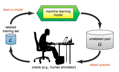
Fig. 1. Active learning
Active learning is an iterative human-in-the-loop training process: one does not start with a fully labeled data set(in contrast to supervised learning), instead one starts with labeling a small fraction of the data (pool $\mathcal{L}$ in Fig.1) and use it to the model like in the supervised learning setup. After the model converges, it will be used to infer on the rest of unlabeled data (pool $\mathcal{U}$ in Fig.1) and we will calculate an uncertainty score for each unlabeled sample and select those “most difficult” samples to be labeled by a human annotator and once the selected samples are labeled, we add those to the labeled training set and retrain the model with the enlarged training set. This iterative process continues until the model reached the desired performance or we run out labeling budget.
Uncertainty is the key factor determining which samples to be labeled in an active learning process. In this post, I will limit the scope to the deep neuron networks for classification problems. Before we dive deeper, let me introduce some notations to be used latter
Notations
| $f$: | deep neural network classifier |
|---|---|
| $w$: | weights of $f$ |
| $D$: | training set |
| $\mathcal{C}$: | set of labels |
| $x$: | an unseen sample |
Let $f$ denote trained on $D$. At the inference time, the there are three commonly used metric to characterize the uncertainty of $f$ on the unseen sample $x$.
Confidence level
Confidence level measures how confident the prediction $f(x)$ is, it is defined as
i.e. the highest class probability.
Margin
Margin measures how certain the model thinks the sample $x$ belongs to one class vs the rest. It is defined as
Entropy
Entropy of the prediction $f(x)$ is calculated as
The term $-\log p(y=c|x, f) = \log \frac{1}{p(y=c|x,f)}$ is called the surprisal of the event $p(y=c|x, f)$. Intuitively, it measures how surprised the model is when the real class label of $x$ is $c$. The smaller the probability $p(y=c|x, f)$ the more surprised the model should be. Therefore, $H(f(x))$ can be thought as expected surprisal when the model sees the real label of $x$. So higher $H(f(x))$ means $f$ is less certain about $x$.
Confidence level, margin and entropy are more or less equivalent notions, i.e. the uncertain data sampled from those measures have high IoU. In the rest of the post, I will use entropy as a measure of uncertainty. In theory, entropy does look like a good measure of uncertainty, but as the internal mechanism neural network itself is very much a black box, we don’t understand how a prediction is made and naturally we don’t understand the uncertainty associated with a prediction.
How robust entropy is as a measure of uncertainty
Robust in this context means
- Samples with high entropy have a interpretable reason to be “difficult” samples.
- Entropy as a measure should withstand randomization, i.e. models trained with different randomization should yield the similar entropy on any samples
- Entropy should change continous with respect to the input. Mathematically speaking, $H(f(x))$ is indeed a continuous function with respect to $x$, what we meant here is that we don’t want sharp change of entropy when we perturb the input by a small noise.
To investigate this problem, I generated 4 clusters of 2d data from the following Gaussians
The data looks like
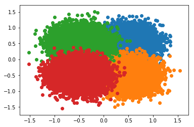
Fig 2. Training data
I then trained a simple fully connect neural net with 5 hidden layers to distinguish those clusters. The model looks like this
import torch
import torch.nn as nn

class DeterministicNet(nn.Module):
    def __init__(self, hidden_layers=5):
        super(DeterministicNet, self).__init__()
        layers = [nn.Linear(2, 10), nn.ReLU(inplace=True)]

        for _ in range(hidden_layers):
            layers.append(nn.Linear(10, 10))
            layers.append(nn.ReLU(inplace=True))

        layers.append(nn.Linear(10, 4))
        self.layers = nn.Sequential(*layers)


    def forward(self, x):
        return self.layers(x)
I call this model DeterministicNet because each neuron is a
deterministic number instead of a random variable. Yes, you guessed right we will talk
about Bayesian network later. Of course we will, how can we avoid Bayesian net when we
are talking about uncertainty?
After 20 epochs of training, the model achieves a humble performance of 95% accuracy on the test set, which is sampled from the exactly the same Gaussians. Ok, now we are happy, because we have a reasonale architecture that can learn the distribution of those clusters. Let’s use it to study the robustness of entropy.
Here is what I did:
- Train 10 models on the same data with different randomization (same hyperparamters)
- Sample 10000 points $S$ uniformly from the 2d plan $[-1.5, 1.5] \times [-1.5, 1.5]$
- Let the 10 trained models to infer on $S$ and plot the entropy of each sample in $S$ as a heatmap.
Here is the result:
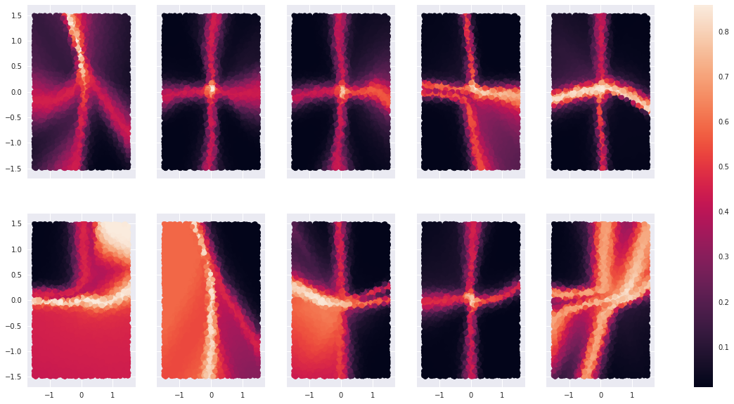
Fig 3. Heatmap-1
Before we start philosophying on this diagram, let’s ask ourselves what heatmap are we expecting? If the model $f$ understands the distribution of the data, then where it should be confused?
I intentionally generated the data in the way so that there are big areas of intersections among clusters. Since those 4 Gaussians are symmetric with respect to the origin and they are the same upto translation, points in the middle of intersection should be the most confusing ones. The heatmap at (1,4) is the one we are expecting.
What does the experiment tell us?
-
Only heatmaps at (1,4) and (2, 5) fullfil our expectation of the distribution of uncertainty. The rest of the models produce inconsistent entropies. That means the quantity $H(f(x))$ does depend on how the model $f$ is trained, and they don’t converge even if the model itself converges.
-
Entropy varies wildly. In many heatmaps in Fig.2, entropy drops shaply immediately outside the axes.
Back to our question, is entropy a good measure of uncertainty?
To the 1st observation, we should realize that uncertainty is in fact a subtle concept. There are two possible sources of uncertainty:
- uncertainty that is inherent in the data itself In the above experiment, data lie in the middle of intersection carries this type of uncertainty. The features of those data are not sufficient for any model, including the homo sapien themselves, to make a confident prediction. Which cluster does $(0, 0)$ belong to? All I say is it belongs to each cluster with a chance of 25%. It is clear that data with inherent uncertainty are useless for training a model.
Another source of uncertainty arises from the model’s lack of “knowledge” in certain regions of the data. In heatmap (2,3), the model lacks “knowledge” about the red cluster. Points near the center of the orange cluster do not carry inherent uncertainty, but the model still cannot cannot understand this region. This is in fact the type of uncertainty we are looking for.
To the 2nd observation, we should take a step back and ask ourself is $f(x)$ itself a mildly continuous function? Meaning does small perturbations to $x$ induce small perturbations in $f(x)$? This question has been studied in the context of adversarial examples. People found that a tiny and visually unperceptable perturbation to an input image can cause the state-of-art CNN to make random predictions. But state-of-art CNNs are hundred-layers deep, the chaotic effects of adding small noise to the input propagates through the layers and becomes even more unfathomably chaotic, that’s why adding small change to the input will cause dramatic change in the prediction. We don’t have this problem for our humble 7-layer perceptron. I resampled uniformly from the 2d-plane and plot the heatmap of entropy of the same 10 models

Fig 4. Heatmap-2
The heatmap, to my eye, is very much the same as in Fig 3. This means our model is fairly stable and the fact that entropy drops shapely outside the axes cannot be attributed to model instability. I think the reason behind it is that the cross entropy loss function encourages the model to make low entropy prediction, so that as soon as the model gains more clue regarding which cluster a sample belongs, it makes a highly confident prediction to minimize the cross entropy loss.
So what have we learnt so far:
- $H(f(x))$ does not distinguish between inherent uncertainty in the data and the model’s lack \ of training on certain distribution
- $H(f(x))$ can change very rapidly
Back to our motivation of using entropy as a measure of uncertainty to sample informative data for active learning, what the above experiment showed is that one could sample data with inherent uncertainty, in which case the training would be frutile; Or one could sample points in a very narrow range, in which case one can drastic increase the variance of the data distribution and cause the training to be unstable.
Let’s verifying this by running an active learning experiment with entropy as a measure of uncertainty. The python-flavored pseudo-code for the experiment is
Init the model
train_set <-  80% data shown in Fig. 2
test_set <- 20% data shown in Fig. 2

# keep track of which samples is labeled
# start by pretending all samples are unlabeled
unlabeled = list(range(len(train_set)); labeled = []

for loop in range(10):
    if loop == 0:
        selected_indices = Randomly Select 1000 samples from `unlabeled`
    else:
        selected_indices = Select 1000 samples from `unlabeled` with the highest entropy

    # add selected samples to the pool of labeled data
    labeled.extend(selected_indices)

    # remove selected samples from the pool of unlabeled data
    unlabeled = unlabeled - selected_indices

    # train the model with labeled data
    train(model, labeled)

    # validate the model on the test set
    validate(model, test_set)
At the end of each loop, we will compute the validation accuracy. We will compare this experiment with a random active learning as the baseline. Random active learning simply means at the begining of each loop, it randomly choose 1000 samples to add to the labeled pool. The result is shown below
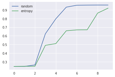
Fig 5. Entropy active learning
$x$-axis indicates the loop number and $y$-axis indicates the validation accuracy. As we can see, the baseline wins by a big margin in the intermediate loops.
Let’s look at what points are being sampled at each loop of the entropy-based active learning
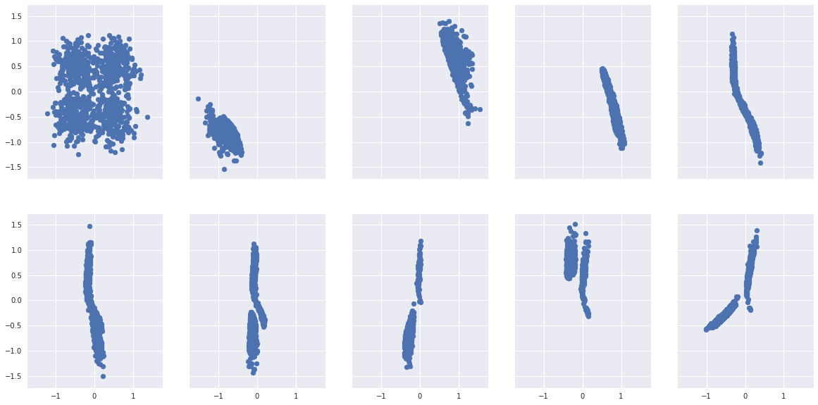
*Fig 6. Points sampled through entropy
It does confirm our using entropy, one can either sample points with inherent uncertainty like in (2, 1), (2,2), (2, 3) or points with narrow range of distribution.
Uncertainty is certainly a reasonable sampling strategy to select informative data, but as we have seen in this post if we don’t choose the right metric to proxy uncertainty, it can lead to bad training result.
In the upcoming posts, I will discuss uncertainty derived from Bayesian framework and why it is a much better way of measuring model’s uncertainty.